

A confusion matrix is a method of summarizing a classification algorithm’s performance. It is simply a summarized table of the number of correct and incorrect predictions.
As you know in supervised machine learning algorithms, we train the model on the training dataset and then use the testing data to make predictions.
For the regression model, we use various matrices including root mean square, mean square, R-square score, etc to evaluate the performance of the regression model.
In the case of a classification model, we use either accuracy, precision, or recall to evaluate the performance of the model.
But there are one more powerful matrices that can be used to show visually how well the classification model was in making predictions and that tool is the confusion matrix. We can also calculate accuracy, precision, and recall using a confusion matrix.
One of the biggest advantages of the confusion matrix is that it gives us a better idea about the miss-classified classes in the classification problems.
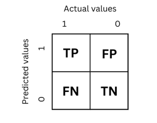
Now let us understand the structure of the confusion matrix in more details before going to the implementation part.
Table of Contents
- What is True Positive (TP)?
- What is True Negative (TN)?
- What is False Positive (FP)?
- What is False Negative (FN)?
- How a confusion matrix works for binary classification?
- Sklearn confusion matrix for binary classification problem
- Sklearn confusion matrix for multi classification problem
- Conclusion
What is True Positive (TP)?
An outcome where the model properly predicted the positive class is referred to as a true positive. In other words, the model forecasts the genuine value.
For instance, if the training dataset contains output classes, let’s say a cat class would stand in for the positive class, and a dog class would stand in for the negative class.
And let’s imagine the input image was a cat, and our model also identified it as a cat. In this case, we would state the value is true positive because both the predicted and the actual values are True.
For example, the below confusion matrix shows the true positive value.
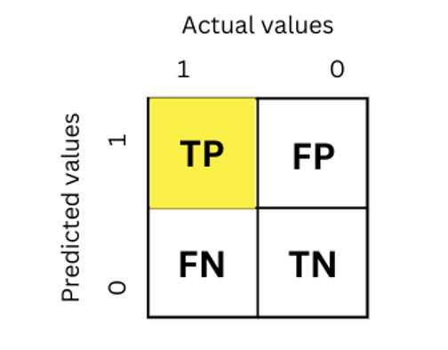
As you can see in the figure above, the TP value is when the actual value was 1 ( positive class) and the predicted value is also 1.
What is True Negative (TN)?
An outcome where the model properly predicted the negative class is referred to as a true negative. In other words, the incorrect value is correctly predicted by the model.
For instance, if the dog class in our training dataset represents a false or negative class, and the model is given an image of a dog to predict, and if it correctly identifies the image as a dog, then we say that the result is a true negative.
Below confusion matrix shows the True Negative value.
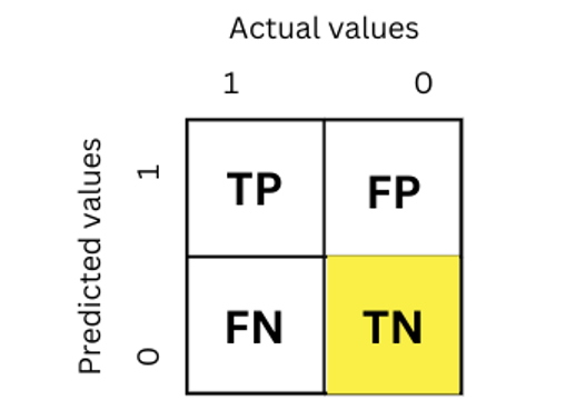
As you can see 0 was the actual value and the prediction is also 0 which mean it is false negative value.
What is False Positive (FP)?
A false positive is a result when the model predicts the positive class inaccurately. In other words, when the model assumes a value to be true, when it is actually a false value is a False
Positive. Using the same dog and cat example, we say that our model made a false positive when it classified the dog image as a cat. The following image shows the false positive value in the confusion matrix.
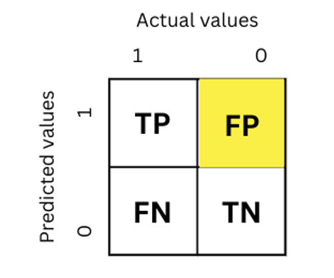
The actual value is 0 and the model predicted it as 1 which mean it is not actual True/Positive class but our model predicted the value to be True/Positive that is why it is called false positive.
What is False Negative (FN)?
A false negative is a result where the model predicts the negative class inaccurately. For instance, we claim it is a False Negative when our model labels an image of a cat as a dog.
In other words, even though a value is predicted by the model to be false, it actually has a True value. The following confusion matrix shows the false negative value.
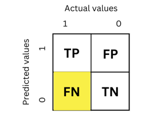
The actual value was 1 but the model predicted it to be 0, so it is false negative.
How a confusion matrix works for binary classification?
Now, let’s jump into the practical part and understand how the confusion matrix works for a binary classification problem.
As we already discussed, for a binary classification the size of the confusion matrix will be 2×2.
The confusion matrix can be used to calculate the accuracy, precision, and f-score which we will learn in a while.
First, let us take an example and discuss how the confusion matrix works for binary classification.
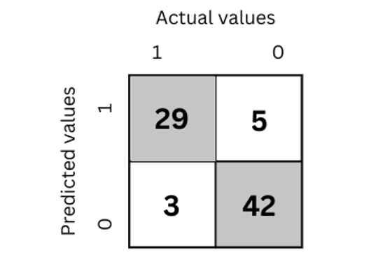
We can get a lot of information from the confusion matrix above. For instance, we can observe that 29 of the 34 true classes were accurately categorized. And 42 out of 45 false classes were classified correctly.
The simplest way to understand a confusion matrix is that everything in the main diagonal represents the correctly classification and the rest all are the errors or miss-classifications of the model.
Let us calculate TP, TN, FP, and FN values from the above confusion matrix because they will help us to calculate accuracy, precision and f1-score.
- True positive values = 20
- True negative values = 42
- False positive values = 5
- False negative values = 3
We can calculate precision, accuracy and f1-score using the following formulae.
- Accuracy = (TP + TN ) / (TP + TN + FP + FN)
- Precision = (TP) / (TP + FP)
- F1-score = (2TP) / ( 2TP + FP + FN)
Sklearn confusion matrix for binary classification problem
Now we will take a simple example and will implement the confusion matrix for binary classification using sklearn module.
We will take the KNN model as an example and will implement it on breast_dataset which is available in sklearn module.
We will not spend too much time understanding the training process of KNN because our main focus is to understand how the confusion matrix works on binary classification.
Let us first load the dataset, train the model on 70% of the dataset and then make predictions for the rest of 30%.
# importing the required modules
from sklearn.datasets import load_breast_cancer
from sklearn.neighbors import KNeighborsClassifier
from sklearn.model_selection import train_test_split
# loading the data
cancer = load_breast_cancer()
# spliting dataset into testing and training parts.
X_train, X_test, Y_train, Y_test = train_test_split(cancer.data,cancer.target, test_size=0.3)

# training the knn model on training parts
knn = KNeighborsClassifier()
knn.fit(X_train, Y_train)

# making predictions on the testing dataset
y_pred = knn.predict(X_test)
In the above code, we trained the KNN model ( which is used for classification problems), and then it predicts the output values on the testing data.
Now, we will use the confusion matrix to visualize how well the predictions were and will use it to calculate the accuracy, precision, and f1-score.
# importing seaborn and matplotlib
import seaborn as sns
import matplotlib.pyplot as plt


# Making the Confusion Matrix
from sklearn.metrics import confusion_matrix

# providing actual and predicted values
cm = confusion_matrix(Y_test, y_pred)

# If True, write the data value in each cell
sns.heatmap(cm,annot=True)

# saving confusion matrix in png form
plt.savefig('confusion_Matrix.png')
Output:
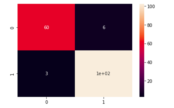
As we know, everything in the main diagonal represents the correctly classified elements, which means only 9 elements have been misclassified by the KNN model.
Let us also calculate the classification report.
# finding the whole report
from sklearn.metrics import classification_report
print(classification_report(Y_test, y_pred))
Output:
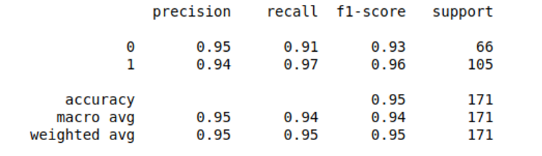
As you can see, the report contains accuracy score, precision, recall, and f1-score.
Sklearn confusion matrix for multi classification problem
Now we will take the dataset about multi-classification and will train the KNN model again. In this section, we will use iris_dataset which is also available in sklearn module.
It contains information about three different types of flowers.
Let us load the dataset, train the model and make predictions about the type of the flower.
# importing the required modules
from sklearn import datasets
from sklearn.neighbors import KNeighborsClassifier
from sklearn.model_selection import train_test_split

iris = datasets.load_iris()

# spliting dataset into testing and training parts.
X_train, X_test, Y_train, Y_test = train_test_split(iris.data,iris.target, test_size=0.3)

# training the knn model on training parts
knn = KNeighborsClassifier()
knn.fit(X_train, Y_train)

# making predictions on the testing dataset
y_pred = knn.predict(X_test)
Now, again we will use the confusion matrix to evaluate the performance of the KNN model for multiclassification problem.
# importing seaborn and matplotlib
import seaborn as sns
import matplotlib.pyplot as plt


# Making the Confusion Matrix
from sklearn.metrics import confusion_matrix

# providing actual and predicted values
cm = confusion_matrix(Y_test, y_pred)

# If True, write the data value in each cell
sns.heatmap(cm,annot=True)

# saving confusion matrix in png form
plt.savefig('confusion_Matrix.png')
Output:
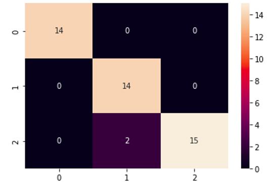
As you can see, this time the confusion matrix is 3×3 because there was a total of 3 output classes.
All the values in the main diagonal represent the correct classification which means only two values were incorrectly classified by the model.
Let us also calculate the classification report.
# finding the whole report
from sklearn.metrics import classification_report
print(classification_report(Y_test, y_pred))
Output:
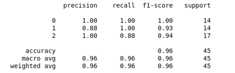
As you can see, we get an accuracy score of 96%.
Conclusion
A confusion matrix is a table that is often used to describe the performance of a classification model (or “classifier”) on a set of test data for which the true values are known.
The confusion matrix itself is relatively simple to understand, but the related terminology can be confusing.
In this article, we discuss how the confusion matrix works and we implemented the confusion matrix using sklearn module.