

Can a machine classify handwritten digits better than the human brain?
Let’s see if Convolutional Neural Networks can give us some insight into this matter, then we’ll let you be the judge.
To add some context for Convolutional Neural Networks, we’ll begin the tutorial with a practical example of a neural network.
A Convolutional Neural Network (CNNs / ConvNets) is a class of deep neural networks, most commonly applied to analyze visual imagery with many applications in image processing.
CNNs have the ability to automatically detect the important features of an object (here an object can be a handwritten character, a face, etc.) without any human supervision or intervention.
In research, it is shown that Deep Learning algorithms such as multilayer CNNs with the use of Keras and Tensorflow offer the highest accuracy compared to other machine learning algorithms such as SVM, KNN & RFC. Due to their high accuracy, CNNs are widely used in image classification, video analysis, etc.
Table of Contents
Dataset
Let’s look at a concrete example of a neural network that uses the Python library Keras to learn to classify and recognize handwritten digits.
The problem we’re trying to solve here is to classify grayscale images of handwritten digits (28 X 28 pixels) into their ten categories (0-9), develop a robust test harness for estimating the performance of the model, use the model to make predictions on new data, and explore improvements to the model.
We will use the MNIST dataset, a classic in the Data Science community which has been intensely studied. It’s a set of 60,000 training images, plus 10,000 test images, assembled by the National Institute of Standards and Technology (the NIST in MNIST) in the 1980s.
As you become a machine learning practitioner, you will see the MNIST dataset come up over and over again, in scientific papers, blog posts, and so on.
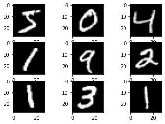
Now before we start, it is important to note that every data point has two parts: an image and a corresponding label describing the actual image, and each image is a 28×28 array, i.e. 784 numbers.
The label of the image is a number between 0 and 9 corresponding to the TensorFlow MNIST image. To download the MNIST Dataset and plot the images, use the following commands:
import tensorflow as tf
from tensorflow.keras.datasets import mnist
from matplotlib import pyplot
(train_images, train_labels), (test_images, test_labels) = mnist.load_data(path="mnist.npz")

#plot images
for i in range(9):
    #define subplot
    pyplot.subplot(330 + 1 + i)
    #plot raw pixel data
    pyplot.imshow(train_images[i], cmap=pyplot.get_cmap('gray'))

#show the figure
pyplot.show()
Output:
The train_images and train_labels form the training set –the data that the model will learn from.
The model will then be tested on the test set comprising of test_images and test_labels.
The images are encoded as NumPy arrays, and the labels are an array of digits, ranging from 0 to 9. The images and labels have a one-to-one correspondence.
Let’s have a look at the shape of the training and test data:
print('Train: Images=%s, Labels=%s' % (train_images.shape, train_labels.shape))
print('Test: Images=%s, Labels=%s' % (test_images.shape, test_labels.shape))
Output:
Train: Images=(60000, 28, 28), Labels=(60000,)
Test: Images=(10000, 28, 28), Labels=(10000,)
Model Building
The workflow will be as follows:
- First, we’ll feed the neural network the training data, train_images, and train_labels.
- The network will then learn to associate images and labels.
- Finally, we’ll ask the network to produce predictions for test_images, and we’ll verify whether these predictions match the labels from test_labels.
Let’s build our model:
from tensorflow.keras.models import Sequential
from tensorflow.keras.layers import Dense, Conv2D, Flatten, MaxPooling2D
model = Sequential()
model.add(Conv2D(32, (3,3), activation = 'relu',input_shape=(28, 28, 1)))
model.add(MaxPooling2D((2, 2)))
model.add(Conv2D(64, (3,3), activation = 'relu'))
model.add(MaxPooling2D((2, 2)))
model.add(Conv2D(64, (3,3), activation = 'relu'))
A ConvNet takes as input tensors of shape (image_height, image_width, image_channels). In this example, we configured the ConvNet to process inputs of size (28, 28, 1), which is the format of the MNIST images.
We did this by passing the argument input_shape = (28, 28, 1) to the first layer. The layer is the core building block of neural networks, it extracts representations out of the data fed into them.
You can think of this term as a filter for your data.
The second and last layer is a 10-way softmax layer, which means it will return an array of 10 probability scores (summing to 1). Each score will be the probability that the current digit image belongs to one of our 10 digit classes.
Let’s display the architecture of the ConvNet so far:
Output:
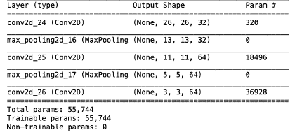
You can see that the output of every Conv2D and MaxPooling2D layer is a 3D tensor of shape (height, width, channels). The width and height dimensions tend to shrink as you go deeper into the network.
Next, we will feed the last output tensor (of shape (3,3,64)) into a densely connected classifier network. These classifiers process vectors, which are 1D, whereas the current output is a 3D tensor.
First, we have to flatten the 3D outputs to 1D, and then add a few Dense layers on top.
model.add(Flatten())
model.add(Dense(64, activation='relu'))
model.add(Dense(10,activation='softmax'))
model.summary()
Output:
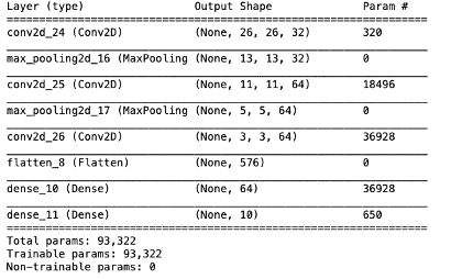
As you can see, the (3,3,64) outputs are flattened into vectors of shape (576,) before going through two Dense layers.
Now, let’s train the ConvNet on the MNIST digits. To make the model ready for training, we need to pick three more things, as part of the compilation process:
- A loss function: this is how we will be able to measure the performance of the model on the training data.
- An optimizer: this is the mechanism through which the model will update itself based on the data it sees and its loss function.
- Metrics: This will be used to monitor the accuracy (the fraction of the images that were correctly classified) of the training and testing model.
Before training, we’ll preprocess the data by reshaping it into the shape the network expects and scaling it so that all values are in the [0,1] interval.
Our training images are stored in an array of shape (60000,28,28) of type uint8 with values in the [0,255] interval. We will transform it into a float32 array of shape (60000, 28 * 28) with values between 0 and 1.
x_train = train_images.reshape(train_images.shape[0], 28, 28, 1)
x_test = test_images.reshape(test_images.shape[0], 28, 28, 1)
input_shape = (28, 28, 1)
x_train = x_train.astype('float32')/255
x_test = x_test.astype('float32')/255
We’re now ready to compile and train the model:
model.compile(optimizer='adam',
              loss='sparse_categorical_crossentropy',
              metrics=['accuracy'])
model.fit(x_train,train_labels, epochs=5)
test_loss, test_acc = model.evaluate(x_test, test_labels)
Output:
313/313 [==============================] - 2s 7ms/step - loss: 0.1085 - accuracy: 0.9892
When this model is evaluated we see that just 5 epochs gave use the accuracy of 98.92% at a very low loss.
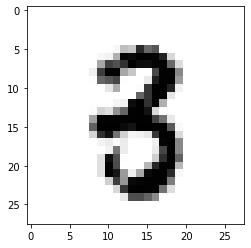
Let’s check its prediction:
image_index = 2853
pyplot.imshow(x_test[image_index].reshape(28, 28),cmap='Greys')
predict = x_test[image_index].reshape(28,28)
pred = model.predict(x_test[image_index].reshape(1, 28, 28, 1))
print(pred.argmax())Output:
Regularization Techniques
The objective of a neural network is to have a final model that performs well both on the data that we used to train it (e.g., the training dataset) and the new data on which the model will be used to make predictions.
However, learning and generalizing to new cases can lead to overfitting or underfitting.
Overfitting is caused by having too few samples to learn from, rendering you unable to train a model that can generalize to new data. Overfitting can be fixed by reducing the number of features in the training data and reducing the complexity of the network through various techniques.
Regularization is a technique that makes slight modifications to the learning algorithm such that the model generalizes better. This in turn improves the model’s performance on the unseen data as well.
L2 Regularization
This regularization is popularly known as weight decay as it forces the weights to decay towards zero (but not exactly zero). This strategy drives the weights closer to the origin by adding the regularization term omega which is defined as:
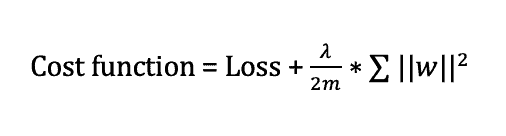
Here, lambda is the regularization parameter. It is the hyperparameter whose value is optimized for better results.
In Keras, we can directly apply regularization to any layer. Let’s apply regularization to our current model:
from tensorflow.keras import regularizers
model = Sequential()
model.add(Conv2D(32, (3,3), activation = 'relu',input_shape=(28, 28, 1)))
model.add(MaxPooling2D((2, 2)))
model.add(Conv2D(64, (3,3), activation = 'relu'))
model.add(MaxPooling2D((2, 2)))
model.add(Conv2D(64, (3,3), activation = 'relu'))
model.add(Flatten())
model.add(Dense(64, activation='relu', kernel_regularizer=regularizers.l2(0.0001)))
model.add(Dense(10,activation='softmax', kernel_regularizer=regularizers.l2(0.0001)))
model.compile(optimizer='adam',
              loss='sparse_categorical_crossentropy',
              metrics=['accuracy'])
model.fit(x_train,train_labels, epochs=5)
test_loss, test_acc = model.evaluate(x_test, test_labels)
Output:
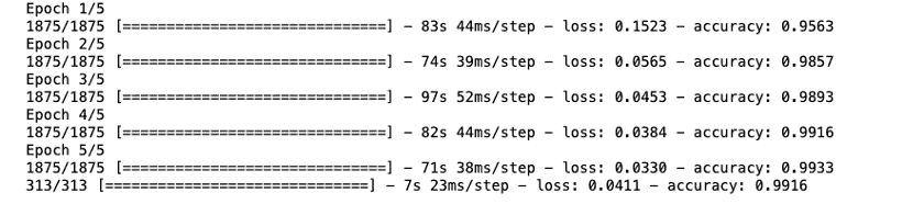
Here the value 0.0001 is the value of the regularization parameter, i.e., lambda.
This showed a little improvement over the previous model. Let’s jump to the dropout technique.
Dropout
Dropout is another interesting regularization technique. At every iteration, it randomly selects some nodes and removes them along with all of their incoming and outgoing connections as shown below.
So each iteration has a different set of nodes and this results in a different set of outputs.
In Keras, we can implement dropout using the Keras core layer.
Below is the python code for it:
from keras.layers import Dropout
model = Sequential()
model.add(Conv2D(32, (3,3), activation = 'relu',input_shape=(28, 28, 1)))
model.add(MaxPooling2D((2, 2)))
model.add(Conv2D(64, (3,3), activation = 'relu'))
model.add(MaxPooling2D((2, 2)))
model.add(Conv2D(64, (3,3), activation = 'relu'))
model.add(Flatten())
model.add(Dropout(0.2))
model.add(Dense(64, activation='relu', kernel_regularizer=regularizers.l2(0.0001)))
model.add(Dense(10,activation='softmax', kernel_regularizer=regularizers.l2(0.0001)))
model.compile(optimizer='adam',
              loss='sparse_categorical_crossentropy',
              metrics=['accuracy'])
model.fit(x_train,train_labels, epochs=5)
test_loss, test_acc = model.evaluate(x_test, test_labels)
Output:
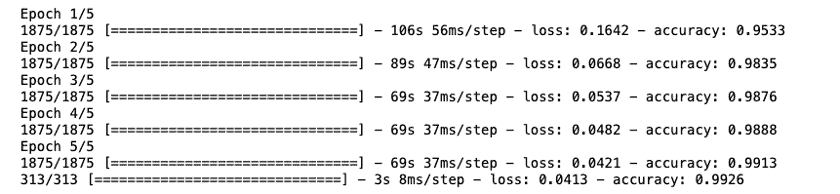
As you can see, we have defined 0.2 as the probability of dropping. This model also showed a little improvement to the previous model.
Data Augmentation
The simplest way to reduce overfitting is to increase the size of the training data. In this case, there are a few ways of increasing the size of the training data –rotating the image, flipping, scaling, shifting, etc.
This technique is known as data augmentation. This usually provides a big leap in improving the accuracy of the model. It can be considered as a mandatory trick in order to improve our predictions.
In Keras, we can perform all of these transformations using ImageDataGenerator. It has a big list of arguments that you can use to pre-process your training data.
from keras.preprocessing.image import ImageDataGenerator
train_datagen = ImageDataGenerator(rotation_range=40,
                            width_shift_range=0.2,
                            height_shift_range=0.2,
                            shear_range=0.2,
                            zoom_range=0.2,
                            horizontal_flip=True,
                            fill_mode='nearest')
train_datagen.fit(x_train)

model = Sequential()
model.add(Conv2D(32, (3,3), activation = 'relu',input_shape=(28, 28, 1)))
model.add(MaxPooling2D((2, 2)))
model.add(Conv2D(64, (3,3), activation = 'relu'))
model.add(MaxPooling2D((2, 2)))
model.add(Conv2D(64, (3,3), activation = 'relu'))
model.add(Flatten())
model.add(Dense(64, activation='relu'))
model.add(Dense(10,activation='softmax'))
model.compile(optimizer='adam',
              loss='sparse_categorical_crossentropy',
              metrics=['accuracy'])
model.fit(x_train,train_labels, epochs=5)
test_loss, test_acc = model.evaluate(x_test, test_labels)
Output:
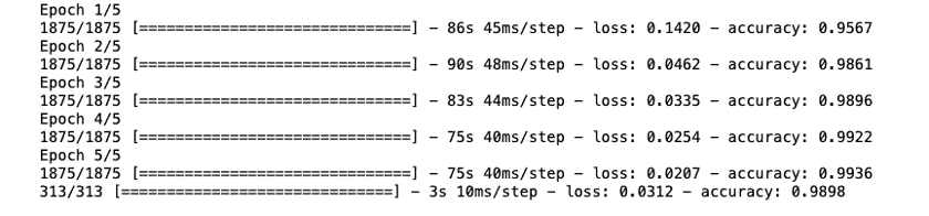
To our surprise, this model did not show any improvement to our basic ConvNet model.
Early stopping
Early stopping is a type of cross-validation strategy where we keep one part of the training set as the validation set. When we see that the performance on the validation set is getting worse, we immediately stop the training on the model.
from keras.callbacks import EarlyStopping
model.compile(optimizer='adam',
loss='sparse_categorical_crossentropy',
metrics=['accuracy'])
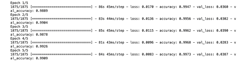
model.fit(x_train,train_labels, epochs=5, validation_data =(x_test, test_labels),
callbacks = [EarlyStopping(monitor = 'val_accuracy', patience = 2)])Output:
Conclusion
You can see that our model stops after only 5 iterations as the validation accuracy was not improving.
It gives good results in cases where we run it for a larger value of epochs. You can say that it’s a technique to optimize the value of the number of epochs.
By far the dropout technique did a better job at recognizing the handwritten digits of the MNIST data compared to the other techniques used.