
In this tutorial we are going to learn about the difference between over-fitting and under-fitting in machine learning with the help of the Python Programming library ScikitLearn, also known as SkLearn.
Table of Contents
- Understanding Undrfitting
- Python Packages
- Data Preparation
- Polynomial Model Fitting and Prediction
- Workflow Simplification Using Pipelines
- Conclusion
Understanding Undrfitting
One important task in machine learning is constructing statistical models. You would like to model the data as accurately as possible, but at the same time realize there is always noise in the data that can lead to overfitting or over-amplification of the noise.
You need to carefully balance between the bias and variance tradeoff.
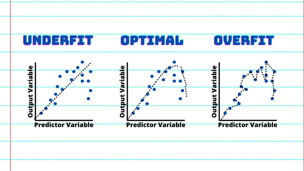
If the model does not have enough parameters to capture the trends in the underlying system, it is called underfitting.
One obvious example is to fit a parabolic curve by a linear function. An underfitting model has a high bias.
On the other hand, if the model has too many parameters, it often leads to overfitting.
One such example is when one tries to model the parabolic curve containing random noises with high order polynomials. The high order polynomial would try hard to fit the noises such that it contains high variance.
Python Packages
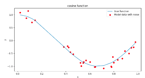
To better understand and compare underfitting and overfitting, let’s study a simple example of the cosine function. We’ll have to first create a sine wave containing random noises and then use different models to fit the experimental data.
We will employ different models that have polynomial features of different degrees to illustrate the effect of overfitting and underfitting when the model we employ contains too many or too few parameters.
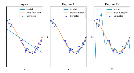
The first model is a linear function (polynomial with degree 1) which will be underfitting due to the lack of enough model parameters.
The second model is a polynomial of degree 4, which will fit the true function almost perfectly.
The third model is a high order polynomial (up to order 15) which will overfit the experimental data by learning too much from the noise in the data. To quantitatively demonstrate the overfitting and underfitting, we will use a cross-validation tool in Python.
Python is probably the most popular and powerful tool for data analysis and machine learning. Python provides all the packages and functions and classes that you can call directly to build and run your own statistical models, including the fitting of models we will demonstrate in this tutorial.
In particular, we will be using both the NumPy and Scikit-learn packages from Python. NumPy is a fundamental scientific package of Python, and Scikit-learn is a very popular Python library for machine learning built on top of NumPy.
Scikit-learn is generally used for implementing regression models, reducing dimensionality, classification models, and clustering models.
Data Preparation
We assume users have already installed Python on your computers. One can import various packages using the following Python code:
import numpy as np
import sklearn as sk
First, we need to generate experimental data. The following Python code generates a cosine function as plotted after the codes. The cosine function is defined and called true_fun which takes a vector X as input and returns the function values cos(1.5 ℼ x) as another vector.
We set the value of n_samples to 30 for the total number of points of our experimental data. Numpy (imported with alias np here) has pre-installed package random that contains most random functions such as rand().
Calling this random number generator rand() with parameter n_samples, x is assigned 30 random points in the range 0 and 1. We call another function sort() in the Numpy package to sort the elements of x in the order of magnitude.
The vector x generated this way is a row vector. As we also need to pass x in the form of the column vector, we call the method new axis in Numpy to convert x from row vector to column vector.
Finally, we compute and store the cosine function for variable x in another vector y_true. In order to demonstrate the overfitting and underfitting, we add random noise to y_true to create real-life cosine data containing normally distributed noise with a mean of 0.1.
def true_fun(X):
    return np.cos(1.5 * np.pi * X)
n_samples = 30
x = np.sort(np.random.rand(n_samples))
# make x from row vector to column vector with shape (30,1)
x_col = x[:,np.newaxis]
# define y from true_fun
y_true = true_fun(x)
# add normal distributed noise with mean 0.1
noise = np.random.randn(n_samples) * 0.1
y = y_true + noise
Polynomial Model Fitting and Prediction
The polynomial regression fitting in Python is actually a linear regression for the polynomials of variables x. This is a smart procedure, but it might confuse beginners. To put in more details, assume we have a 1-dimension variable vector x = [1,2,3,4,5].
Instead of training a polynomial regression model on x directly (which is numerically difficult and slow), the Python polynomial regression actually trains a linear regression model on all polynomials on x.
E.g. the 3rd-order (or degree 3) polynomial transformation on the above vector x becomes [ [1,1,1], [2,4,8], [3,9,27], [4,16,64[, [5,25,125]], i.e. each value of vector x is now transformed to [x,x^2,x^3].
Following such polynomial transformation, a simple linear regression on the new polynomial variables [x,x^2,x^3,…] is performed to compute the linear coefficient slope for x, x^2, x^3, etc.
The Python code below illustrates how to prepare the degree 4 polynomial regression features and then perform linear regression fitting and prediction.
# import polynomial regression and linear regression models
from sklearn.preprocessing import PolynomialFeatures
from sklearn.linear_model import LinearRegression
# define instances from the above model classes
polynomial = PolynomialFeatures(degree=4)
linear = LinearRegression()
# polynomial fitting and transform to x_poly
x_poly = polynomial.fit_transform(x_col)
# perform linear regression between x_poly and y
linear.fit(x_poly,y)
# predict using the linear regression object linear_reg
y_pred = linear.predict(x_test)
Now we test the above code for degree=1 (linear model), degree=4 (4th order polynomial regression), and degree=15 (15th high order polynomial fitting).
The plots below show the predicted y values for different degree values. It is clearly observed that degree=1 leads to underfitting (i.e. trying to fit cosine function using linear polynomial y = b + mx only), while degree=15 leads to overfitting (i.e. using a 15th order polynomial to fit the cosine function).
Workflow Simplification Using Pipelines
In the above Python codes, we have to repeatedly cast data into specific forms in order to perform polynomial fitting, transform, and linear regression prediction.
In addition, in order to evaluate the accuracy of various model fitting and analyze overfitting, one needs to use Python modules model_selection which provides functions for evaluating the cross-validation and analysis.
In Python, one can simplify this whole workflow using a pipeline structure.
In the codes below, we use the pipeline module to do polynomial regression fitting and prediction together with model evaluation. The parameter scoring in the cross_val_score provides different types of scoring such as root-mean-square error, average, accuracy, etc.
The parameter cv determines the cross-validation splitting strategy. Setting cv=5, for example, creates a 5-fold sub-sets from the original data for computing the statistical bias and variance.
from sklearn.pipeline import Pipeline
from sklearn.model_selection import cross_val_score
pipeline = Pipeline([("polynomial_features", polynomial),
                     ("Linear regression", linear)])
# fit to x_col
pipeline.fit(x_col, y)
# predict y_pred
y_pred = pipeline.predict(x_test)
# Evaluate the models using cross validation
scores = cross_val_score (pipeline, x_col, y,
                          scoring='neg_mean_squared_error', cv=5)
If we print the scores for the three polynomial regression models, the mean-squared-errors for degree=1, 4, 15 are 1.02, 5.75, and 9.8e+14 respectively!
The polynomial regression model using 15th-order polynomial leads to overfitting resulting in a huge mean-square-error of 9.8e+14!
Conclusion
This article introduces the common terms of overfitting and underfitting, which are the two opposing extremes but both result in poor performance in machine learning. Overfitting in the polynomial regression usually happens to a model that was trained too much on the particulars and noises of the training data.
A model that is overfitting will not perform well on new data. On the other hand, underfitting typically refers to a model that has not been trained sufficiently such as using a linear model to fit a quadratic function.
A model that is underfitting will perform poorly on the training data as well as new data alike. In order to find the sweet spot in between, people often use pipelines to test on multiple models and compute the cross validation for each model to help select the optimal model.
This is where the model performs well on both training data and new testing data.