

A time series is a sequence of data points collected over time. In many domains, there is always a need to deal with multivariate time series data, such as a network of sensors measuring weather conditions, or multiple financial indices reflecting global economics.
Due to the nature of non-stationary and complicated correlation, it is a hard challenge to analyze and forecast a multivariate time series.
Table of Contents
Introduction to Keras
In this tutorial, we will illustrate how to analyze multivariate time series using Keras, which is a very popular and powerful deep learning framework for Python. Keras is a high-level neural network API written in Python that can provide convenient ways to define and train almost any kind of deep learning model. Keras is capable of running on top of Tensorflow, Theano, and CNTK.
Predicting Stock Prices
Stock prices depend on many factors, and it is a good example to illustrate how we can use Keras in Python to predict the stock market with multivariate time series. Of course, the ideal prediction (and almost impossible) needs one to take into account all the possible factors that affect the stock market.
In this article, we treat the stock price time series as a high-dimensional image. Consider if we collect N days of historical stock prices, and then slice it into many smaller segments, e.g. each segment containing only 100 days of historical stock prices.
Then, we stack all the (N-100) segments together which yields a time series of N-100 variables that is ready for neural network training through Keras.
Below is a step-by-step code implementation and explanation beginning with installing the correct ancillary package for gathering our data:
pip install pandas-datareaderLoad data
Collection and cleaning of data is usually the first and most time-consuming part, other than the training.
In this example, we load all the price data on the NASDAQ composite index from finance.yahoo.com into our Python project. We use DataReader provided by pandas, a fundamentally important package in Python, to download the data from the Yahoo website.
import numpy as np
import pandas_datareader.data as web

# Getting NASDAQ quotes whose symbol is IXIC
df = web.DataReader('^IXIC', start="2010-01-01",end="2020-06-01", data_source="yahoo")
df
The pandas DataFrame of the NASDAQ looks like the following table:
| Date | High | Low | Open | Close | Volume | Adj Close |
|---|---|---|---|---|---|---|
| 2010-01-04 | 2311.149902 | 2294.409912 | 2294.409912 | 2308.419922 | 1931380000 | 2308.419922 |
| 2010-01-05 | 2313.729980 | 2295.620117 | 2307.270020 | 2308.709961 | 2367860000 | 2308.709961 |
| 2010-01-06 | 2314.070068 | 2295.679932 | 2307.709961 | 2301.090088 | 2253340000 | 2301.090088 |
| 2010-01-07 | 2301.300049 | 2285.219971 | 2298.090088 | 2300.050049 | 2270050000 | 2300.050049 |
| 2010-01-08 | 2317.600098 | 2290.610107 | 2292.239990 | 2317.169922 | 2145390000 | 2317.169922 |
| … | … | … | … | … | … | … |
| 2020-05-26 | 9501.209961 | 9333.160156 | 9501.209961 | 9340.219727 | 4432310000 | 9340.219727 |
| 2020-05-27 | 9414.620117 | 9144.280273 | 9346.120117 | 9412.360352 | 4462450000 | 9412.360352 |
| 2020-05-28 | 9523.639648 | 9345.280273 | 9392.990234 | 9368.990234 | 4064220000 | 9368.990234 |
| 2020-05-29 | 9505.549805 | 9324.730469 | 9382.349609 | 9489.870117 | 4710060000 | 9489.870117 |
| 2020-06-01 | 9571.280273 | 9462.320312 | 9471.419922 | 9552.049805 | 3824770000 | 9552.049805 |
Transform the Data
To fit into the neural network training, the data must be reshaped so that it can feed into the neural network pipeline. We choose a simple way to transform the data, through slicing and stacking.
The original full-length dataset has dimension N x 6, where N is the total number of days of stock trading. If we choose to import stock price data between 2010 and 2020, then N has the length of 10 years of trading days.
While 6 refers to the number of features contained in the stock price dataset, namely the opening price, closing price, and adjusted closing price, the high and low price, and volume.
We choose a value for segment length, say 100, to slice the whole time series so that the data is transformed to the dimensionality of (N-100)*100*6, where N-100 is the number of sliced segments of length 100 from the total N-day series.
Lastly, we need to split the completely transformed dataset into training and testing sets, which is the common practice for most machine learning algorithms. The training dataset is used to train the algorithm and compute the coefficients (or weights) in the approximating functions, and the testing dataset is used to test the accuracy of the algorithm with trained coefficients.
The code below shows how to do this using Python:
segment_length = 100

# Split into training data sets
# choose 80% as training, and 20% as testing dataset
train_data_len = dataset.shape[0] * 0.8
train_data = dataset[0:train_data_len, :]
x_train, y_train = [], []
for i in range(segment_length , train_data_len):
    x_train.append(dataset[i-sequence_length:i,:])
   y_train.append(dataset[i, 0])

# Create the test data
test_data_len = dataset.shape[0] * 0.2
test_data = dataset[train_data_len:, :]
x_train, y_train = [], []
for i in range(train_data_len, train_data_len+test_data_len):
    x_train.append(dataset[i:,:])
    y_train.append(dataset[i, 0])
Training of Multivariate Prediction Model
Now the original raw dataset has been pre-processed and split into training and testing subsets.
We now need to train the model using the training dataset. By choosing our parameters such as the number of input neurons. Such choices are usually up to the experience and dataset.
Next, we’ll import and create an instance of the Sequential() method from the Keras module. The Sequential method is a commonly used model for neural networks. We can add different layers to the neural networks using the add() method in the Sequential model.
After constructing the model, we need to compile it using the compile function in the Sequential model.
# Deep learning library, used for neural networks
from keras.models import Sequential
model = Sequential()
n_neurons = x_train.shape[1] * x_train.shape[2]
model.add(LSTM(n_neurons, return_sequences=False,
               input_shape=(x_train.shape[1], x_train.shape[2])))
model.add(Dense(1, activation='relu'))
# Compile the model
model.compile(optimizer='adam', loss='mean_squared_error')
In the compile method, the user has to decide on various parameters.
The first parameter optimizer is actually not just integral to Keras but a general concept used in Neural Networks. The whole training process in the neural network is to find the optimized weights that yield the best accuracy or robustness. The weights are initially initialized randomly.
In each iteration (or called epoch in Neural Networks), the weights are updated such that the overall accuracy of the network is improved. To measure the output, we need to define and compute the loss functions to compare.
This is essentially an optimization problem where the goal is to optimize the loss function and arrive at ideal weights. The method used for optimization is known as Optimizer.
Gradient Descent is one of the most widely known methods, but there are many others also available in Keras. To name a few, some commonly used ones are SGD, RMSprop, Adam, Adadelta, etc.
We will not go into too much detail. In our code, we choose the Adam optimizer and choose mean-squared error as the loss function.
# Training the model
epochs = 5
early_stop = EarlyStopping(monitor='loss', patience=2, verbose=1)
history = model.fit(x_train, y_train, batch_size=16,
                    epochs=epochs, callbacks=[early_stop])
The above few lines perform the actual training, or fitting, of the model. There are numerous parameters to explore and play with.
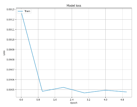
It suffices to know at this level that the value of epochs refers to the number of iterations. The larger the epoch value, the more computational time is needed. We usually choose a value where a good convergence has been reached.
For our dataset, we run the code and plot the loss function vs. epoch in the plot below. For this case, the loss function can be considered converging after 3 iterations, so it’s fine to choose epoch=3.
Prediction using the model
The model can now be used to predict the future stock price after training. The prediction can be implemented easily using the Keras provided predict() method.
predictions = model.predict(x_test)To estimate how accurate the prediction is, we can compute the mean-square error since we actually know the stock price in the y_test (i.e., we compare y_predict with y_test).
MAPE = np.mean((np.abs(np.subtract(y_test, predictions)/ y_test))) * 100
MDAPE = np.median((np.abs(np.subtract(y_test, predictions)/ y_test)) ) * 100
Depending on the parameters, the mean and median error can vary, but we compute the errors to be around 20%.
This is not surprising, as the multivariate model we implemented here only considers the stock price history itself. To accurately predict stock prices, we really need to consider millions of factors in economics.
Conclusion
In this tutorial, we introduced multivariate time series forecasting, by definition all the way to Python implementation.
We used the Keras package which provides an easy way to train a neural network and then fit a model for prediction. Though we used the stock price dataset for our prediction the prediction accuracy was only about 20%; which is not surprising as the true prediction of the stock price is very difficult to predict without all the possible influencing factors in economics.
The point of this tutorial is to illustrate how to prepare and transform our stock market dataset, train, then fit the model by adjusting multiple parameters.
Finally, we’ve also shown how to evaluate our model’s performance by computing and comparing the mean and median errors. The best way to master multivariate time series forecasting is to experiment with different models and their corresponding parameters.
Depending on the nature of the datasets you are interested in, there are no single optimal sets of parameters and models.