Data sets come in different states, shapes, and sizes. When you gain access to a dataset for the first time, there is an element of mystery there. Do all of the records have valid data? Are there any unusual measurements? How large is the dataset?
There is some basic information it would be helpful to know about your dataset before embarking upon deeper analysis. The process of answering these preliminary questions is called “exploratory data analysis.” In this article, we will take a detailed look at exploratory data analysis and conduct our own exploratory data analysis on a public dataset.
Let’s start with building a mental model for the concept of exploratory data analysis by thinking about a visit to the doctor’s office.
Table of Contents
- Data Collection in Real-life
- Sizing Up Your Dataset
- Setting Up the Code
- Installing Modules
- Getting the Dataset
- Dataset Visualization
- Multivariate Data Exploration – Scatter Plots
- Conclusion
Data Collection in Real-life
When you visit your doctor for a check-up, you go through a process before seeing the doctor. An assistant calls you from the waiting room, then proceeds to record a few data points about your state. These data points often include your temperature, pulse, and blood pressure. This group of data points give your healthcare professionals a high-level overview of your health status at that moment.
Without this information, your real-time health status would be a mystery. Depending on your status, certain deep analysis techniques like collecting blood samples for testing could be dangerous. To avoid that kind of risk, the assistant starts by collecting a preliminary set of data points that are non-invasive and easy to obtain. This gives the healthcare professionals a starting point and a better understanding of subsequent steps that can be taken.
Sizing Up Your Dataset
So how does having vital signs collected at a doctor’s visit relate to exploratory data analysis? The process of collecting a preliminary set of data points before seeing the doctor is a form of exploratory analysis. Just as the assistant starts by running lightweight analysis on your health status at the doctor’s office, you can run lightweight analysis on new datasets before conducting more heavy-duty processing.
Exploratory data analysis is a collection of basic tools you can use to gain a basic understanding of a dataset. The two main categories of exploratory data analysis are data visualizations and descriptive statistics. In this article, we will use Python tools and a public dataset to conduct our own data analysis.
Setting Up the Code
Let’s go ahead and get our development environment set up for our exploratory data analysis. In this article, we will be using a Linux system with version 3.8.7 of Python already installed. If you need help installing Python 3 on your system, here is a good resource to help:
For Windows:
For Mac and Linux
It is fine if you install a version of Python that comes after version 3.8.7.
Now, let’s create a directory for our project:
mkdir exploratory_data_analysis

cd exploratory_data_analysis
The system we are using for this project has multiple versions of Python installed, so we will need to use a virtual environment. We can create and activate a virtual environment named venv with version 3.8.7 of Python by running the following commands:
python3.8 -m venv venv

source venv/bin/activate
We can verify that we are running version 3.8.7 in the virtual environment by starting up the Python 3 interactive shell:
python3

exit()
As pictured above, you can exit out of the interactive shell by running the exit() command.
Installing Modules
We will be using the pandas and matplotlib modules.
Let’s start by installing the pandas module using the pip package installer.
pip install pandasAfter the module installation process completes, run pip freeze to see all of the dependencies that were installed on your system as part of the pandas module installation.
pip freeze

pandas==1.2.4
Now that we have pandas on our system, we just need to install matplotlib. Similar to the previous installation step, you can install the matplotlib module by running the following command:
pip install matplotlibLet’s run pip freeze once again after the installation process completes to verify that we have matplotlib on our system.
matplotlib==3.4.1
pandas==1.2.4
As you can see, we have matplotlib version 3.4.1 available.
Now that we have our libraries installed on our system, it is time to set up the dataset.
Getting the Dataset
The dataset we will be using in this article is the “Iris Plants” dataset created by R.A. Fisher. This dataset is publicly available in various places. We downloaded a version of this dataset by searching for the “Iris Species” dataset that was posted by UCI Machine Learning from Kaggle (download below):
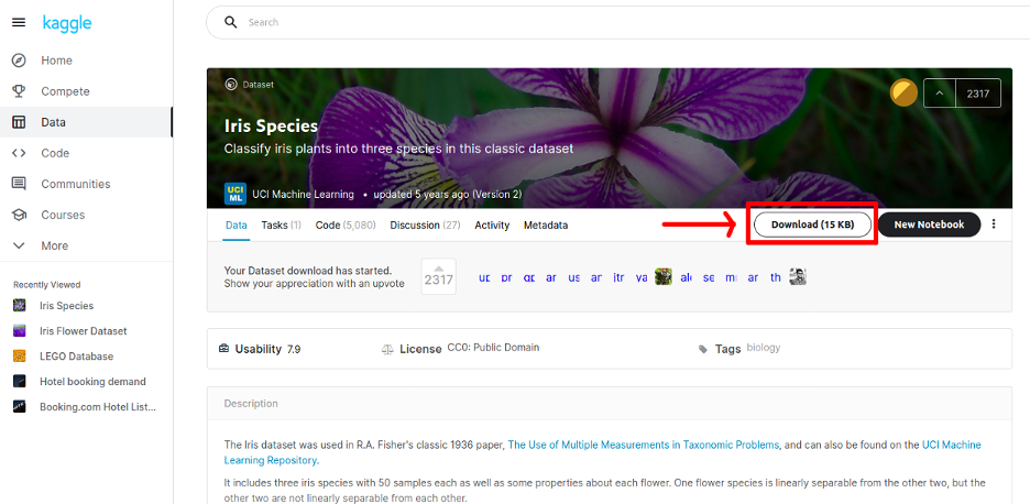
The file download from Kaggle is a zip file that includes a CSV file named Iris.csv. Move your dataset file into the exploratory_data_analysis folder and create a Python script named data_analysis.py.
touch data_analysis.py
ls
data_analysis.py Iris.csv venv
We will import this file into the Python script to begin conducting our exploratory data analysis. In order to do this, we need to import the pandas module into our script.
Once we do that, we can import the CSV file data into our script as pandas DataFrames.
import pandas as pd

# Import CSV data
data_frames = pd.read_csv (r'Iris.csv')

print(data_frames)
If you run the script above, you will see an abbreviated print out of the DataFrames that contain the dataset.
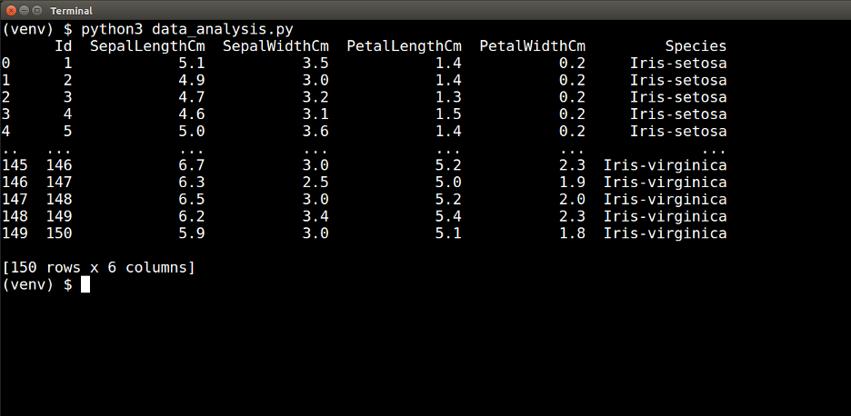
Great! Now that we have our dataset imported into our script, we can start our exploratory data analysis by generating visualizations of the dataset.
Dataset Visualization
Data visualization is the process of generating graphical representations such as graphs, plots, and charts of a dataset. By converting data into a graphical format, it is possible to quickly comprehend patterns via visual analysis.
If we look back at the print out of the imported data above, we will see that this dataset has six attributes (or columns): Id, SepalLengthCm, SepalWidthCm, PetalLengthCm, PetalWidthCm, and Species.
A good way to start familiarizing ourselves with this dataset is to visualize an individual attribute of the data. This is univariate data exploration.
Univariate Data Exploration – Histogram
Let’s explore the SepalLengthCm attribute. There are several rows in this dataset. How can we quickly understand which sepal lengths are common and which ones are rarer? We can generate a histogram to visualize how the different sepal lengths are distributed across the dataset.
To do this, we will need to create another Python script in which we import the matplotlib module. Then we can go ahead and plot a histogram using the values from the SepalLengthCm attribute.
import pandas as pd
import matplotlib.pyplot as plt

# Import CSV data
data_frames = pd.read_csv (r'Iris.csv')

# Plot histogram with sepal length values
plt.hist(data_frames['SepalLengthCm'])

# Label the axes
plt.xlabel('Sepal Length (cm)')
plt.ylabel('Frequency')

# Display
plt.show()
When you run the script above, you will generate a histogram that looks like this:
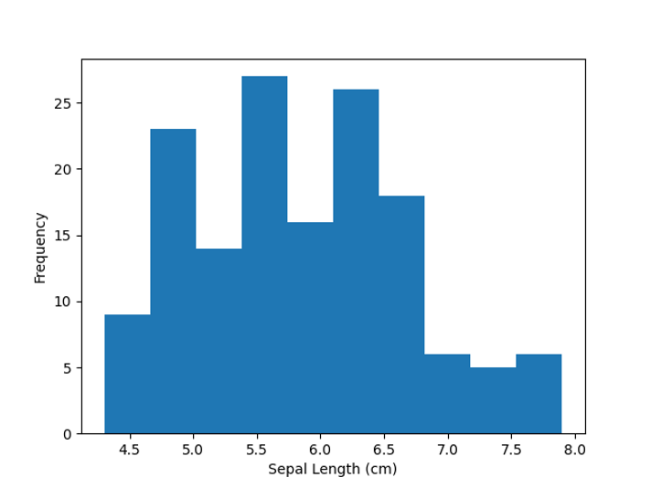
Just by looking at this data visualization, we can immediately identify certain characteristics about this dataset. We see that the sepal lengths range in value from roughly 4.5 cm to somewhere between 7.5 cm and 8.0 cm.
We can also see that after about 6.5 cm, there is a sharp drop in the occurrence of longer sepal lengths.
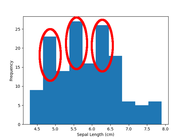
Other characteristics that immediately stand out are the three spikes in sepal length frequency just below 5 cm, around 5.5 cm, and just below 6.5 cm. This observation begs the question – is there a relationship between the sepal length and any of the other data attributes? We can dive into that question when we look at multivariate analysis.
As you can see, this one visual representation of the sepal length values helped us to quickly get to know several things about this dataset. We learned about the range of values, frequency of certain values, and noted a pattern that may be related to other attributes in the dataset.
The matplotlib.pyplot.hist function is highly customizable. We used the default settings here, but it is possible to change various aspects of the graph. Here is a link to the documentation for this particular function: https://matplotlib.org/stable/api/_as_gen/matplotlib.pyplot.hist.html
Multivariate Data Exploration – Scatter Plots
In contrast to univariate data exploration, multivariate data exploration is the analysis of more than one attribute at the same time.
Earlier, we mentioned there may be a relationship between the sepal length and the species. Let’s generate a visualization that shows both of those attributes together with the use of a scatter plot.
import pandas as pd
import matplotlib.pyplot as plt

# Import CSV data
data_frames = pd.read_csv (r'Iris.csv')

# Set values for axes
x = data_frames['SepalLengthCm']
y = data_frames['Species']

# Draw scatter plot
plt.scatter(x, y, c='green')

# Label the axes
plt.xlabel('Sepal Length (cm)')
plt.ylabel('Species')

# Display
plt.show()
When we run this script, we will generate the following plot:
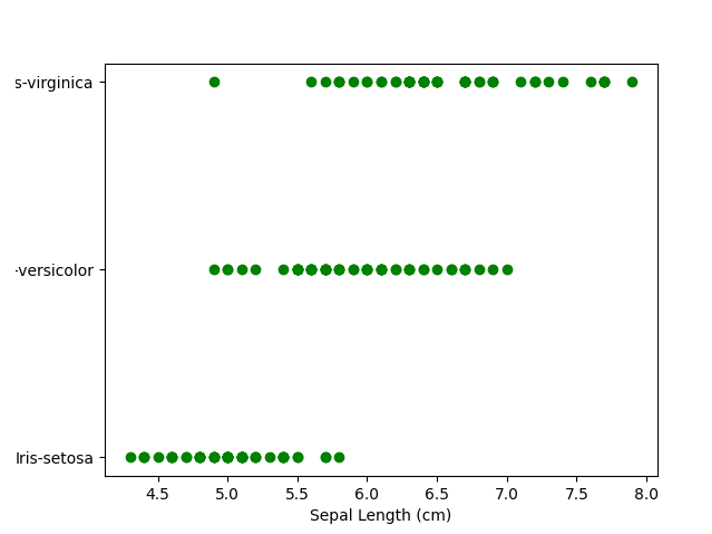
Based on this scatter plot, we can see that the species of Iris flower does have some impact on the sepal length.
For example, we would expect the smallest sepal lengths to come from the setosa species, while the largest sepal lengths come from the virginica species. Overall, however, there is quite a bit of overlap in sepal lengths between the species.
Multivariate Data Exploration – Pie Charts
The next script will generate a pie chart based on how many sepal length measurements there are in the dataset for each species. First we group the SepalLengthCm attribute by the Species.
Then we count the number of sepal length records in each group. In order to determine the values for the labels of the pie chart, we create a DataFrame of the three unique species values.
import pandas as pd
import matplotlib.pyplot as plt

# Import CSV data
data_frames = pd.read_csv (r'Iris.csv')

# Get total count of sepal lengths by species
sepal_lengths_counts = data_frames.groupby(['Species'])['SepalLengthCm'].count()
species = data_frames['Species'].unique()

# Plot pie chart
plt.pie(sepal_lengths_counts, labels=species, colors=['r','g','b'],
    startangle=90, autopct='%1.1f%%')


# Display
plt.show()
When you run the script above, you will generate a pie chart where the total number of sepal length records for each species is the same.
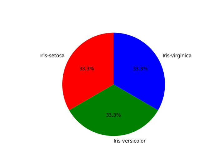
This lets us know that no species is overrepresented in the dataset.
Descriptive Statistics
Descriptive statistics compress key characteristics of a dataset into single values. There are statistics to represent the central tendency of the data, the spread of the values in the dataset, and more.
In this article, we will focus on descriptive statistics for the central tendency and spread of values in a dataset.
Central Tendency and Value Spread
Computing the central tendency of a dataset includes generating statistics such as the mean, median, and mode. These statistics are measures of the middle of the dataset and a value trend across the dataset.
Value spread, on the other hand, is a check on the breadth of values represented in the dataset. When determining the spread of a dataset, you look for minimums, maximums, variance, and standard deviation.
There is one particular function available in the pandas library that calculates and returns most of this information. This function, called describe(), can be called on a pandas DataFrame. It can be run on an individual attribute or the entire dataset.
We will run this function on one attribute, the SepalLengthCm. Create another Python script and enter the code below in order to print out the collection of computed statistics.
import pandas as pd

# Import CSV data
data_frames = pd.read_csv (r'Iris.csv')

print(data_frames['SepalLengthCm'].describe())
In the table below, you see a count, mean, standard deviation, minimum, maximum, and percentiles for the SepalLengthCm attribute.
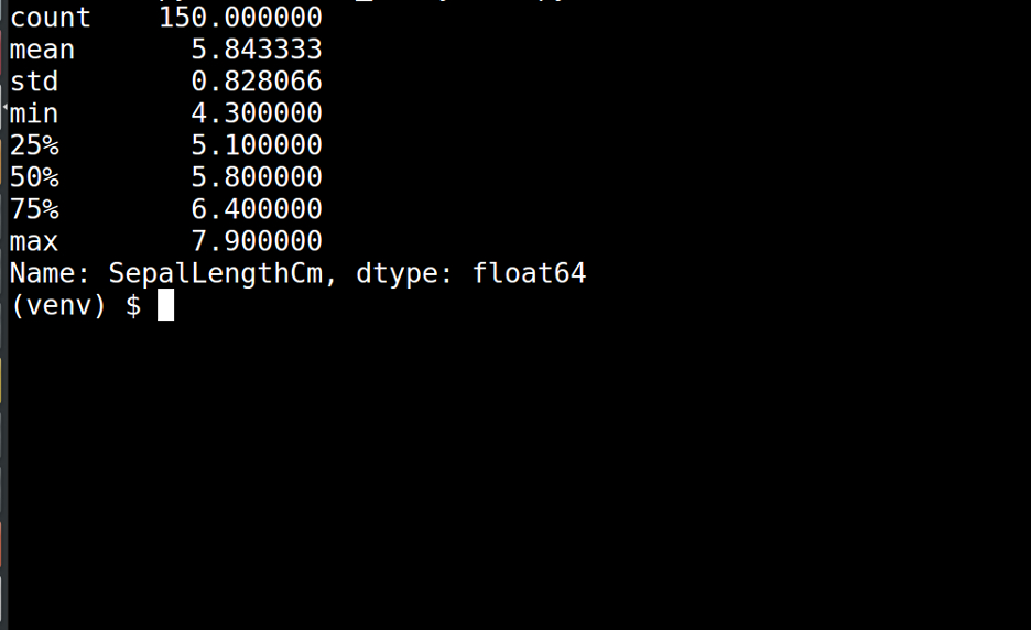
This one tool took care of computing most of the descriptive statistics we wanted, but we still need the median, mode, and variance.
Calculating the median and mode is as simple as calling the functions displayed in the script below:
import pandas as pd

# Import CSV data
data_frames = pd.read_csv (r'Iris.csv')

# Print out the median
print("+--------------+")
print("    Median")
print("+--------------+")
print(data_frames['SepalLengthCm'].median())

# Print out the mode
print("+--------------+")
print("    Mode")
print("+--------------+")
print(data_frames['SepalLengthCm'].mode())
Running this script produces the output displayed below. The median is 5.8, and the mode is 5.0. (Note: the mode is displayed in a one-row table where the row has an id of 0.)
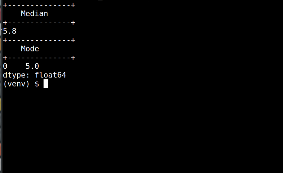
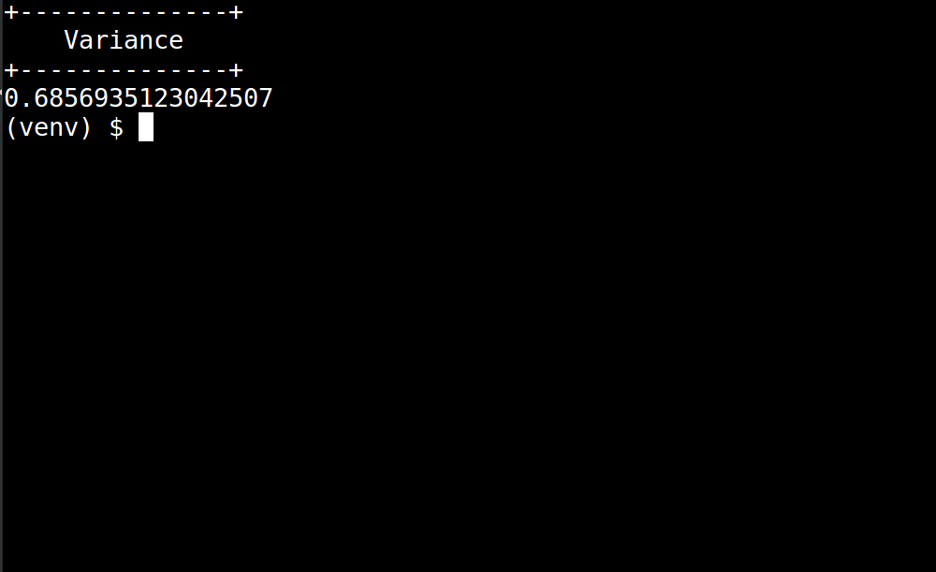
Finally, we need to calculate the variance. The variance of the SepalLengthCm attribute can be calculated by running the following script:
import pandas as pd

# Import CSV data
data_frames = pd.read_csv (r'Iris.csv')

# Print out the variance
print("+--------------+")
print("    Variance")
print("+--------------+")
print(data_frames.var()['SepalLengthCm'])
Here is the output of running the script listed above:
Conclusion
In this article, we looked at the process of exploratory data analysis. Exploratory data analysis involves using a range of tools and measurements, including data visualization and descriptive statistics, to get a feel for a new dataset.
This process is an important step to move from being unfamiliar with a particular dataset to quickly having an idea of the types of additional analysis that would be most productive using that dataset.


